Disease gradient information provides the spatial distribution of the epidemics at distance from the focus. If you are interested in learning how to calculate the area under the disease gradient curve to make comparison of several scenarios or treatments, this would be a good resource.
I am using Steven Worthington’s ipak function to install and load several packages in R.
ipak <- function(pkg){
    new.pkg <- pkg[!(pkg %in% installed.packages()[, "Package"])]
    if (length(new.pkg))
        install.packages(new.pkg, dependencies = TRUE)
    sapply(pkg, require, character.only = TRUE)
}

# usage
packages <- c("tidyverse", "readxl", "agricolae", "ggpubr", "ggpubr", "magrittr", "reshape", "knitr")
ipak(packages)
## Loading required package: tidyverse
## Warning: package 'tidyverse' was built under R version 3.6.3
## -- Attaching packages ----------------------------------------------------- tidyverse 1.3.0 --
## v ggplot2 3.3.2     v purrr   0.3.4
## v tibble  3.0.1     v dplyr   1.0.0
## v tidyr   1.1.0     v stringr 1.4.0
## v readr   1.3.1     v forcats 0.5.0
## Warning: package 'ggplot2' was built under R version 3.6.3
## Warning: package 'tibble' was built under R version 3.6.3
## Warning: package 'tidyr' was built under R version 3.6.3
## Warning: package 'readr' was built under R version 3.6.3
## Warning: package 'purrr' was built under R version 3.6.3
## Warning: package 'dplyr' was built under R version 3.6.3
## Warning: package 'stringr' was built under R version 3.6.3
## Warning: package 'forcats' was built under R version 3.6.3
## -- Conflicts -------------------------------------------------------- tidyverse_conflicts() --
## x dplyr::filter() masks stats::filter()
## x dplyr::lag()    masks stats::lag()
## Loading required package: readxl
## Warning: package 'readxl' was built under R version 3.6.3
## Loading required package: agricolae
## Warning: package 'agricolae' was built under R version 3.6.3
## Loading required package: ggpubr
## Warning: package 'ggpubr' was built under R version 3.6.3
## Loading required package: magrittr
## Warning: package 'magrittr' was built under R version 3.6.3
##
## Attaching package: 'magrittr'
## The following object is masked from 'package:purrr':
##
##     set_names
## The following object is masked from 'package:tidyr':
##
##     extract
## Loading required package: reshape
## Warning: package 'reshape' was built under R version 3.6.3
##
## Attaching package: 'reshape'
## The following object is masked from 'package:dplyr':
##
##     rename
## The following objects are masked from 'package:tidyr':
##
##     expand, smiths
## Loading required package: knitr
## Warning: package 'knitr' was built under R version 3.6.3
## tidyverse    readxl agricolae    ggpubr    ggpubr  magrittr   reshape     knitr
##      TRUE      TRUE      TRUE      TRUE      TRUE      TRUE      TRUE      TRUE

data <- read_excel("field observation.xlsx") %>%
        as.data.frame()
head(data, 10)
##    Distance Treatments     R1      R2    R3    R4
## 1        10         T4  0.375  0.0125  1.75  1.75
## 2        15         T4  0.750  0.0175  1.25  2.50
## 3        20         T4  2.500  1.2500  2.50  3.75
## 4        25         T4  2.750  2.5000  3.75  6.25
## 5        30         T4  2.500  5.0000  3.50 12.50
## 6        35         T4  3.500  6.2500  4.25 15.00
## 7        40         T4  3.000 12.5000  7.50 17.50
## 8        45         T4  5.500 17.5000  6.25 27.50
## 9        50         T4 10.000 27.5000 12.50 30.00
## 10       55         T4 10.000 30.0000 14.00 18.00
audpc_data <- data %>%
  melt(id=c("Distance", "Treatments")) %>%
  group_by(Treatments, variable) %>%
  summarize(AUDPC = audpc(value, Distance))
## `summarise()` regrouping output by 'Treatments' (override with `.groups` argument)

audpc_data %>%
  spread(variable, AUDPC) %>%
  arrange(Treatments) %>%
kable() | Treatments | R1 | R2 | R3 | R4 |
|---|---|---|---|---|
| T1 | 526.39750 | 1200.5000 | 870.7500 | 2288.125 |
| T2 | 24.03125 | 526.2663 | 31.0325 | 1110.938 |
| T3 | 69.95000 | 486.1637 | 247.7063 | 1790.225 |
| T4 | 363.34375 | 894.3062 | 388.7125 | 1078.750 |
| T6 | 0.00000 | 0.0100 | 0.0000 | 0.000 |
| T7 | 0.00250 | 0.0000 | 0.0000 | 0.000 |
plot_graph <- ggplot(audpc_data, aes(Treatments, AUDPC))+
  geom_boxplot(aes(fill=factor(Treatments))) +
  ggtitle("AUDPC")+
  xlab("Treatment Applied")+
  ylab("Area Under Disease Gradient")+
  theme_bw(base_size = 14)+
  theme(aspect.ratio=1.25,plot.title = element_text(hjust = 0.5),
        panel.grid=element_blank())+
  scale_fill_manual(name="Treatments",
                    breaks = c("T1", "T2",
                               "T3", "T4", "T5",
                               "T6", "T7"),
                    labels=c("T1=Inoculated control", "T2=CP culling at 3 days", "T3=CP cull 'ring' x 3","T4=CP cull at 1 day","T5=FP of CP at 3 days","T6=CP cull + FP of non-CP","T7=FP of entire plot at 3 days"),
                    values=c("#999999","#E69F00","#56B4E9", "#009E73", "#F0E442", "#0072B2", "#D55E00"))


plot_graph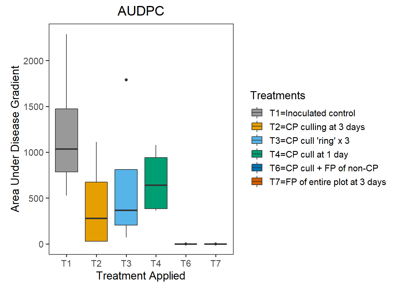
ggsave(filename = "Boxplot.png", width = , height = , units = "in",
       dpi = 600, limitsize = TRUE)
## Saving 7 x 5 in image